LLM Evals Course Lesson 3: Building Automated Evaluators

The third lesson of Hamel Husain and Shreya Shankar’s LLM evaluation course moved from manual error analysis into automated evaluation systems. This session focused on the “Measure” phase of their evaluation lifecycle - how to build evaluators that can automatically detect the failure modes we identified through error analysis.

In terms of the Three Gulfs Model from lesson one, this lesson first helps us distinguish between specification failures (where we need to improve our prompts) and generalisation failures (where the LLM struggles despite clear instructions). The automated evaluators we build specifically target the Gulf of Generalisation, measuring how well our LLM applies instructions across diverse inputs.

They continued using NurtureBoss (an AI leasing agent for apartment complexes) as their running example. Through error analysis in the previous lesson, they’d identified failure modes like hallucinated tool invocations, missing visual information for amenities, and unhelpful responses to ambiguous queries.

Specification vs Generalisation Failures

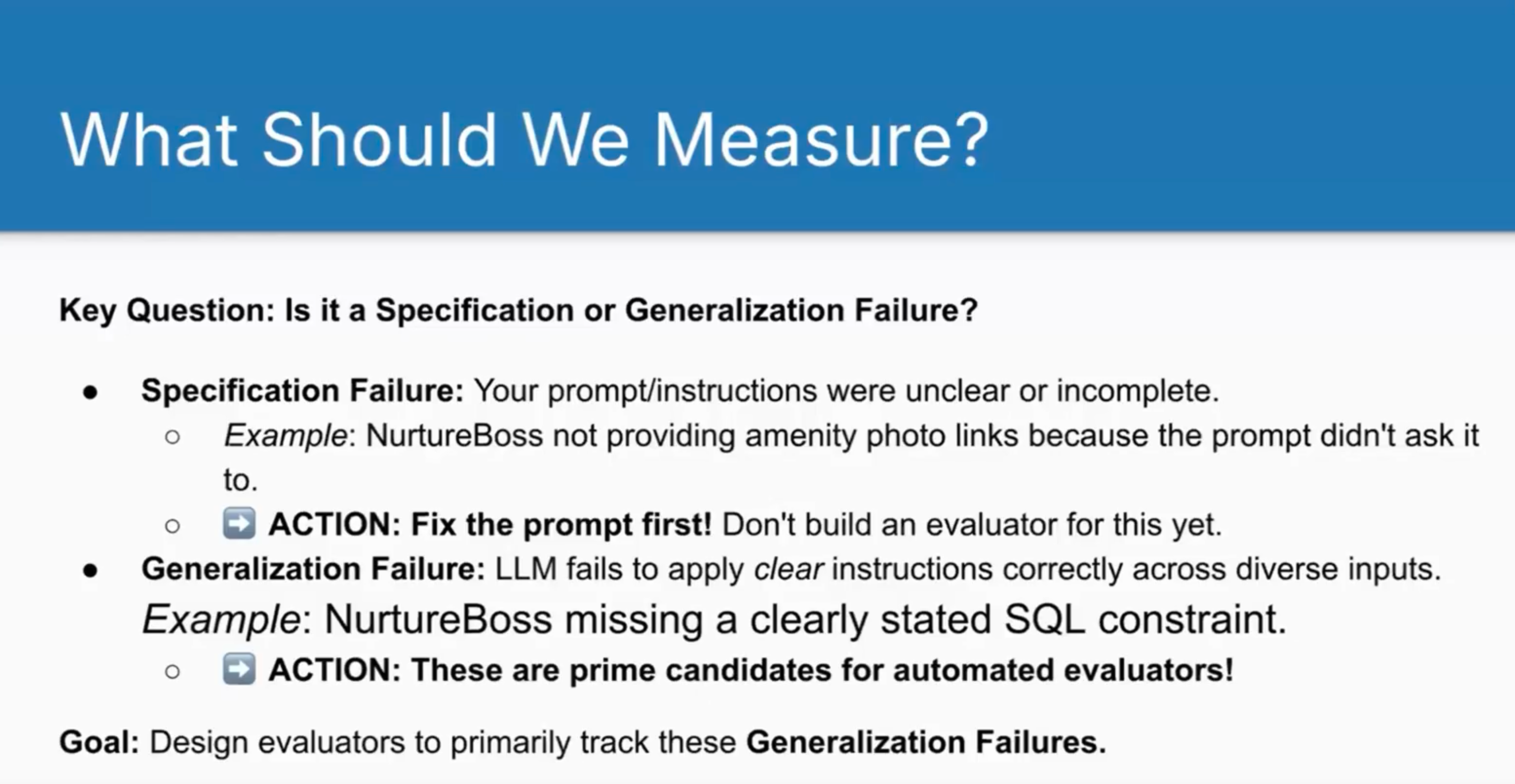
Specification failures occur when your prompt didn’t include sufficient instructions. For example, Shreya realised during error analysis that when advertising a flat with a pool, the system should include photographs. But she’d never specified this in the prompt - the LLM wasn’t failing, it simply hadn’t been told to do this.

Generalisation failures happen when you did provide clear instructions but the LLM fails to apply them correctly across diverse inputs. If you told it to use specific tools and it hallucinates non-existent ones, or if you specified SQL constraints that it ignores, those are generalisation failures.

Specification failures are easy to fix (or at least easy to respond to) - you just update your prompts. It’s not worth building automated evaluators for them. You should build automated evaluators only for generalisation failures, where the LLM genuinely struggles despite clear instructions.

Code-Based vs LLM-as-Judge Evaluators

The course presents two approaches to automated evaluation:

Code-Based Evaluators

These are straightforward programmatic checks for objective, rule-based criteria. They’re fast, cheap, deterministic, and interpretable.

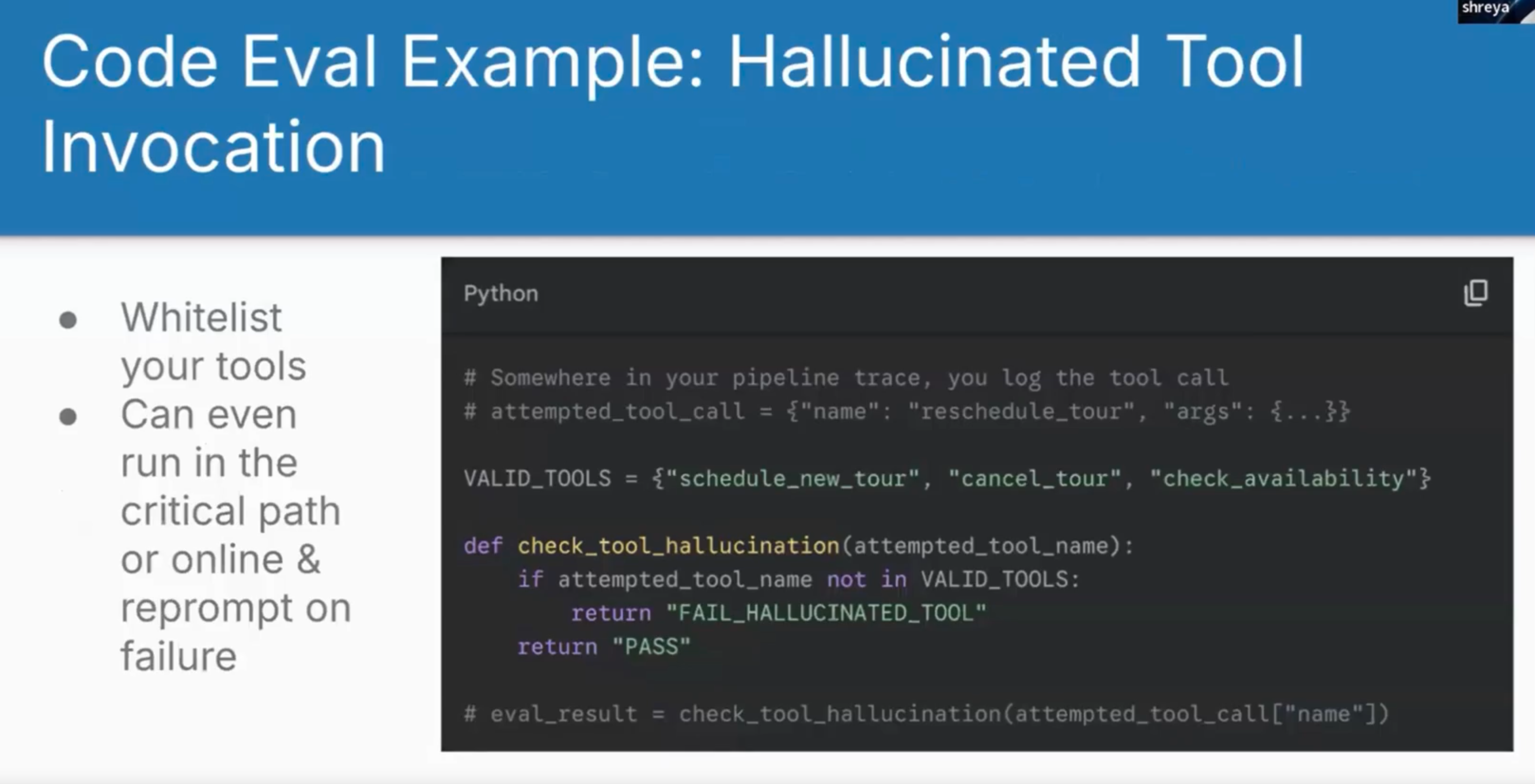
# Somewhere in your pipeline trace, you log the tool call
# attempted_tool_call = {"name": "reschedule_tour", "args": {...}}

VALID_TOOLS = {"schedule_new_tour", "cancel_tour", "check_availability"}

def check_tool_hallucination(attempted_tool_name):
    if attempted_tool_name not in VALID_TOOLS:
        return "FAIL_HALLUCINATED_TOOL"
    return "PASS"

# eval_result = check_tool_hallucination(attempted_tool_call["name"])

I.e., the above code can detect hallucinations, deterministically and cheaply with no LLMs.

Common use cases include:

• Parsing structure (JSON validity, SQL syntax)
• Regex/string matching for keywords
• Structural constraints (exactly three bullet points)
• Tool execution errors

Hamel emphasised pushing yourself to use code-based evaluators wherever possible. Folk love reaching for LLM-as-judge for everything but code-based checks avoid the complexity and cost of validating a judge model.

LLM-as-Judge Evaluators

When your failure modes involve subjectivity, nuance, or complex interpretation that code can’t handle, you need LLM-as-judge. This means using another LLM to evaluate your main pipeline’s outputs.

You should focus each judge on a single, narrowly defined failure mode. Don’t ask “is this good?” or try to evaluate multiple criteria at once. Binary pass/fail decisions on specific aspects make judges more reliable.

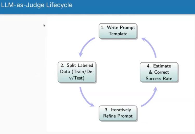
Building a Reliable LLM Judge

The process mirrors building any LLM application, but it’s easier because you’ve scoped the task narrowly. Here’s the lifecycle:

1. Write the Prompt Template

Your judge prompt needs four key components:

1. Clear task and evaluation criterion - Focus on one specific failure mode
2. Precise pass/fail definitions - Explicitly define what constitutes each outcome
3. Few-shot examples - Crucial for calibrating the judge with clear pass and fail cases
4. Structured output format - JSON or XML for easy parsing

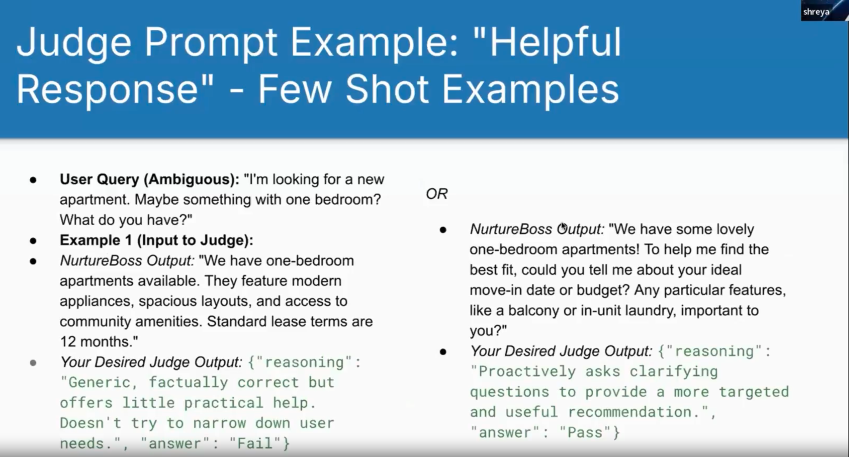
For the “unhelpful response” failure mode, they defined:

• FAIL: Response is generic, passive, provides minimal new information despite ambiguity
• PASS: Response acknowledges ambiguity and proactively attempts to clarify needs

2. Split Your Labelled Data

This is where many people go wrong. You need proper data hygiene with three distinct splits:

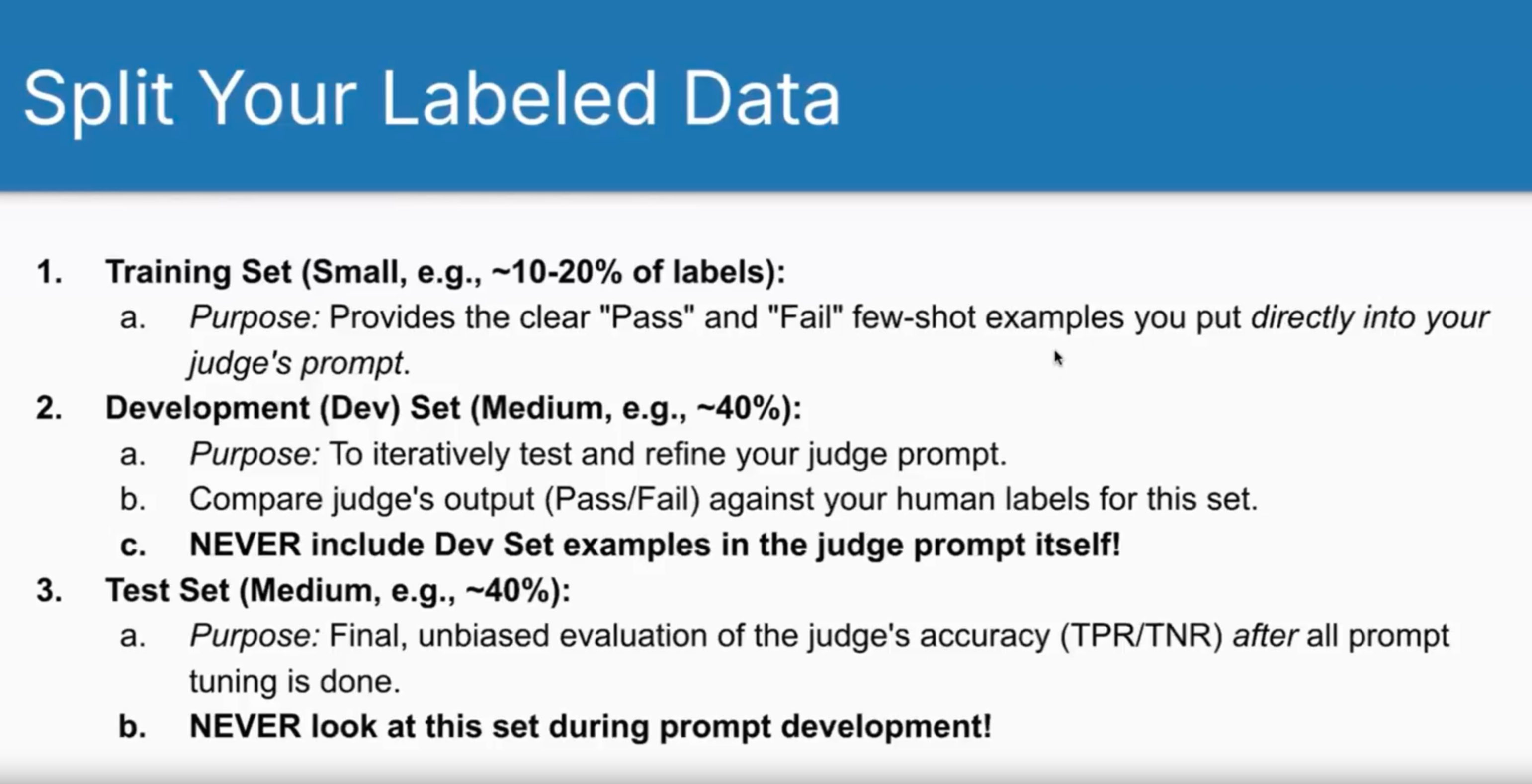
• “Training set” (10-20%): Few-shot examples that go directly in your prompt (it’s not real training - but it’s doing the same job basically)
• Development set (40%): For iteratively refining your judge
• Test set (40%): Final unbiased evaluation - never look at this during development

Shreya said that 90% of people make the mistake of including dev set examples in their judge prompt, which makes accuracy metrics meaningless. I want to think that’s an exaggeration.

3. Iteratively Refine the Prompt

The refinement process focuses on aligning your judge with human labels on the dev set:

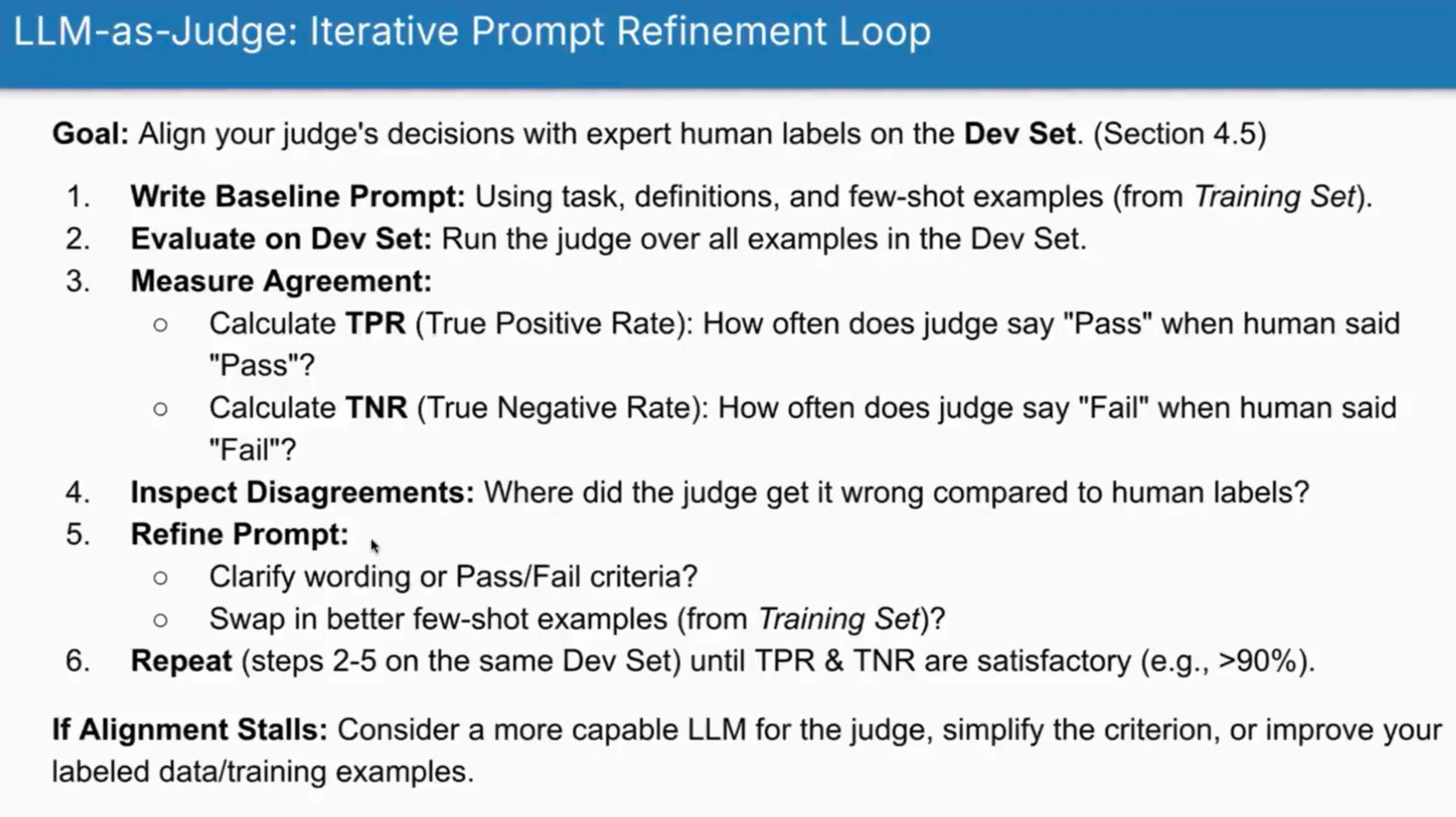
1. Write baseline prompt with task, definitions, and training examples
2. Evaluate on dev set
3. Measure True Positive Rate (TPR) and True Negative Rate (TNR)
4. Inspect disagreements between judge and human labels
5. Refine prompt - clarify definitions, swap examples
6. Repeat until TPR and TNR exceed 90%

It may not be immediately obvious why we use TPR and TNR instead of raw accuracy. Raw accuracy seems intuitively to capture what we’re looking for but it can be skewed by the actual characteristics of your data. For example, if your data has only 10% failures and you always predict “pass”, you’d have 90% accuracy but zero ability to detect actual problems.

4. Estimate and Correct Success Rates

Even good judges aren’t perfect. Their imperfections create bias in the metrics they produce.

The lesson attempted to teach a statistical approach to correct for this bias but I think it got tied up and muddled a bit - it was a bit of a jump to go from high level discussion to stats and formulas with no theoretical grounding in the base concepts.

I found the explanations weren’t particularly clear - here’s my best attempt to explain it. Imagine you want to know what percentage of your AI’s outputs are actually good. You build an LLM judge to evaluate thousands of outputs automatically. But your judge isn’t perfect - maybe when a human would say “this is good”, your judge only agrees 90% of the time (90% TPR), and when a human would say “this is bad”, your judge agrees 85% of the time (85% TNR).

If you run this imperfect judge on 10,000 outputs and it says 82% are good, can you trust that number? Not directly - your judge has systematic biases. The bias correction formula essentially adjusts for these known tendencies, like calibrating a scale that always reads 2kg too heavy.

The confidence intervals tell you the range where the true value likely sits. Instead of falsely claiming “exactly 82% of outputs are good”, you can say “we’re 95% confident it’s between 83% and 87%”. This matters when you’re trying to hit quality targets or measure whether changes actually improved your system.

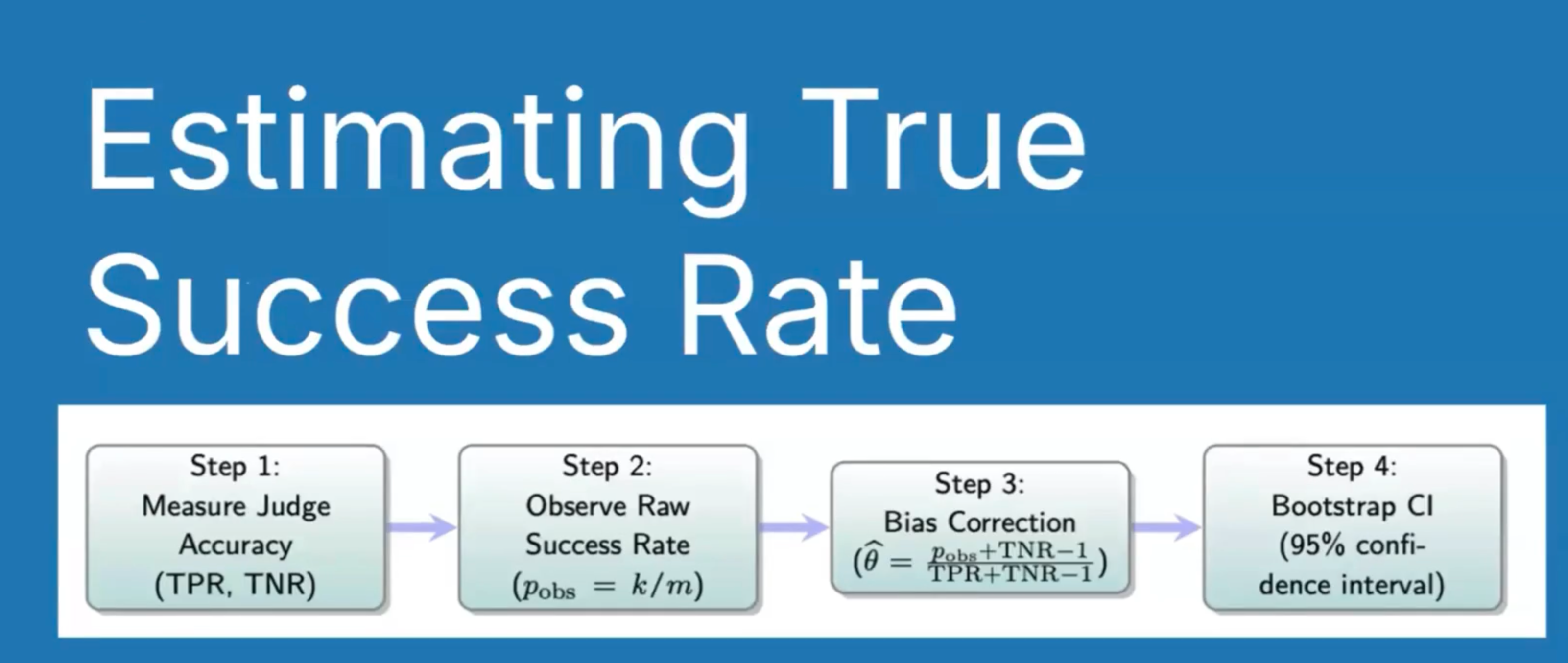
The four-step process:

1. Measure final judge accuracy (TPR/TNR) on test set
2. Run judge on unlabelled production data
3. Apply bias correction formula using known TPR/TNR
4. Calculate confidence intervals through bootstrapping

In this context, bootstrapping is a statistical technique for estimating uncertainty.

Specifically for the LLM judge:

You have a test set where you know both:

• What your judge said (pass/fail)
• What the human labels were (pass/fail)

Bootstrapping means:

1. Randomly resample your test set with replacement (so some examples might appear twice, others not at all)
2. Recalculate TPR and TNR for this resampled set
3. Apply the bias correction formula using these new TPR/TNR values
4. Repeat this process many times (say 1000 times)

You end up with 1000 different estimates of the true success rate. The spread of these estimates tells you about uncertainty:

• Take the 2.5th percentile and 97.5th percentile of all these estimates
• This gives you a 95% confidence interval

Why “bootstrapping”?

It’s called “bootstrapping” because you’re using your existing data to simulate what would happen if you collected new test sets many times. You’re “pulling yourself up by your bootstraps” - using the data you have to understand the variability in your estimates.

Instead of just saying “our success rate is 85%”, you can say “we’re 95% confident it’s between 83% and 87%”, which is much more honest about the uncertainty in your measurement.

Judge errors primarily inflate uncertainty (wider confidence intervals) rather than shifting the estimate itself. To get tighter bounds, focus on improving TPR - the judge’s ability to correctly identify successes.

Real-World Impact of Judge Quality

The course included several visualisations showing how judge quality affects estimates in different scenarios:

Scenario 1: Good Judge but Limited Labels

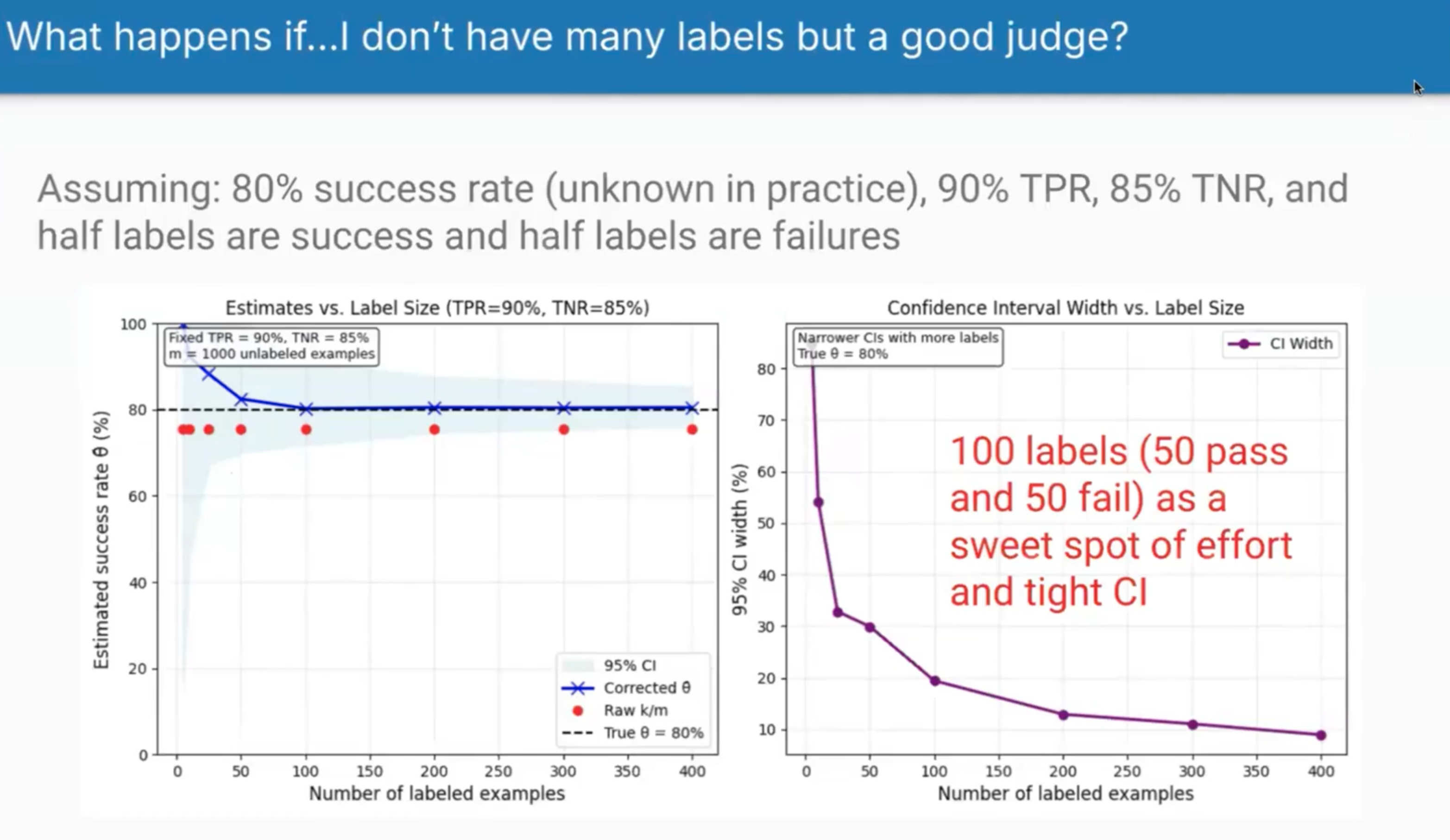
When you have a decent judge (90% TPR, 85% TNR) but varying amounts of labelled data, two things happen. First, the raw judge estimates (red dots) consistently underestimate the true 80% success rate because the judge is slightly too critical. Second, as you add more labelled examples, the confidence intervals narrow dramatically. They found 100 labels to be the sweet spot - enough to get reliable estimates without excessive labelling effort.

Scenario 2: Poor at Identifying Success

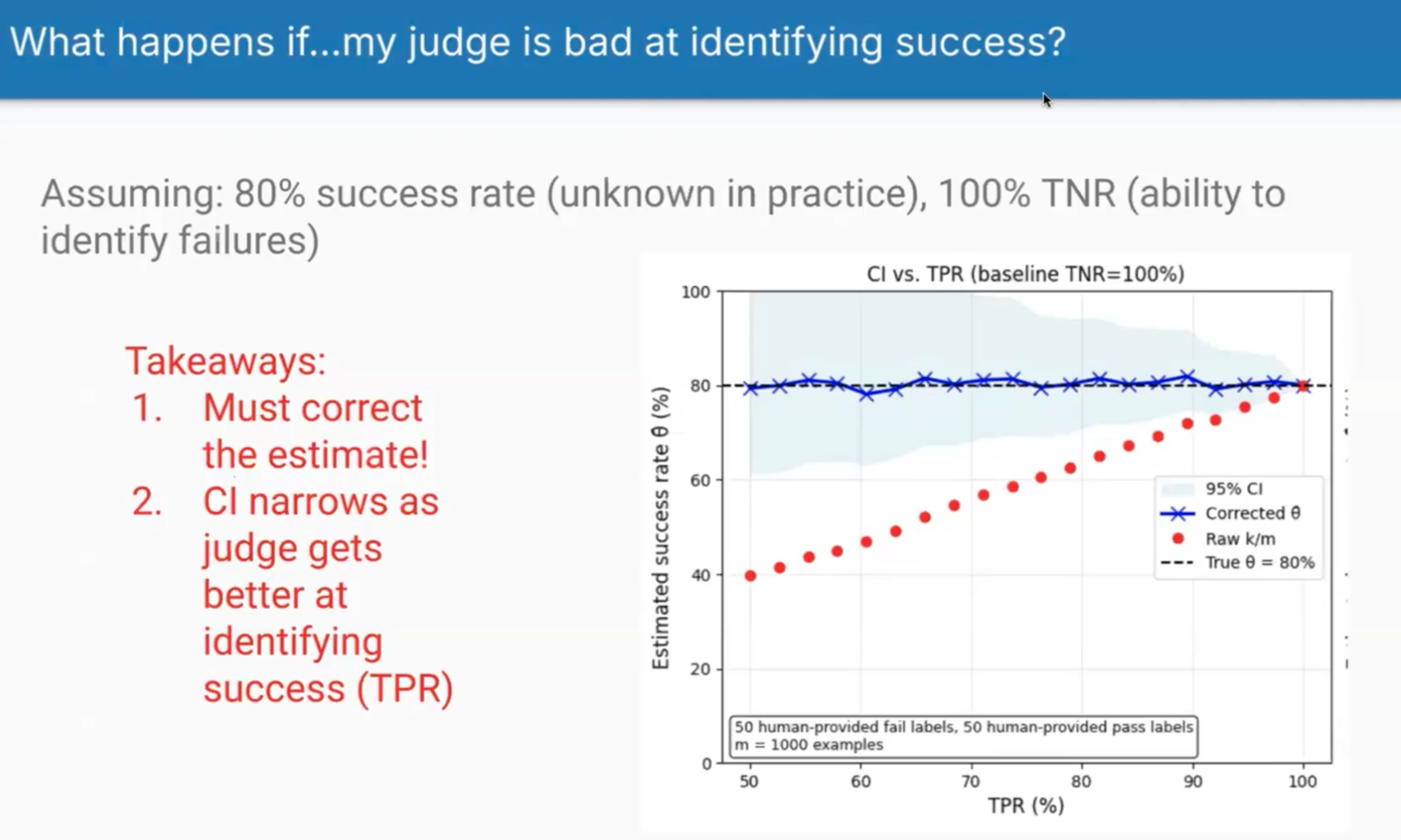
This shows what happens when your judge struggles to recognise successes (varying TPR) but perfectly identifies failures (100% TNR). The gap between raw estimates and reality is massive when TPR is low - if your judge only recognises 60% of successes, it will dramatically underestimate your system’s performance. The bias correction helps, but the key lesson is that improving your judge’s ability to recognise successes has the biggest impact on accuracy.

Scenario 3: Poor at Identifying Failures

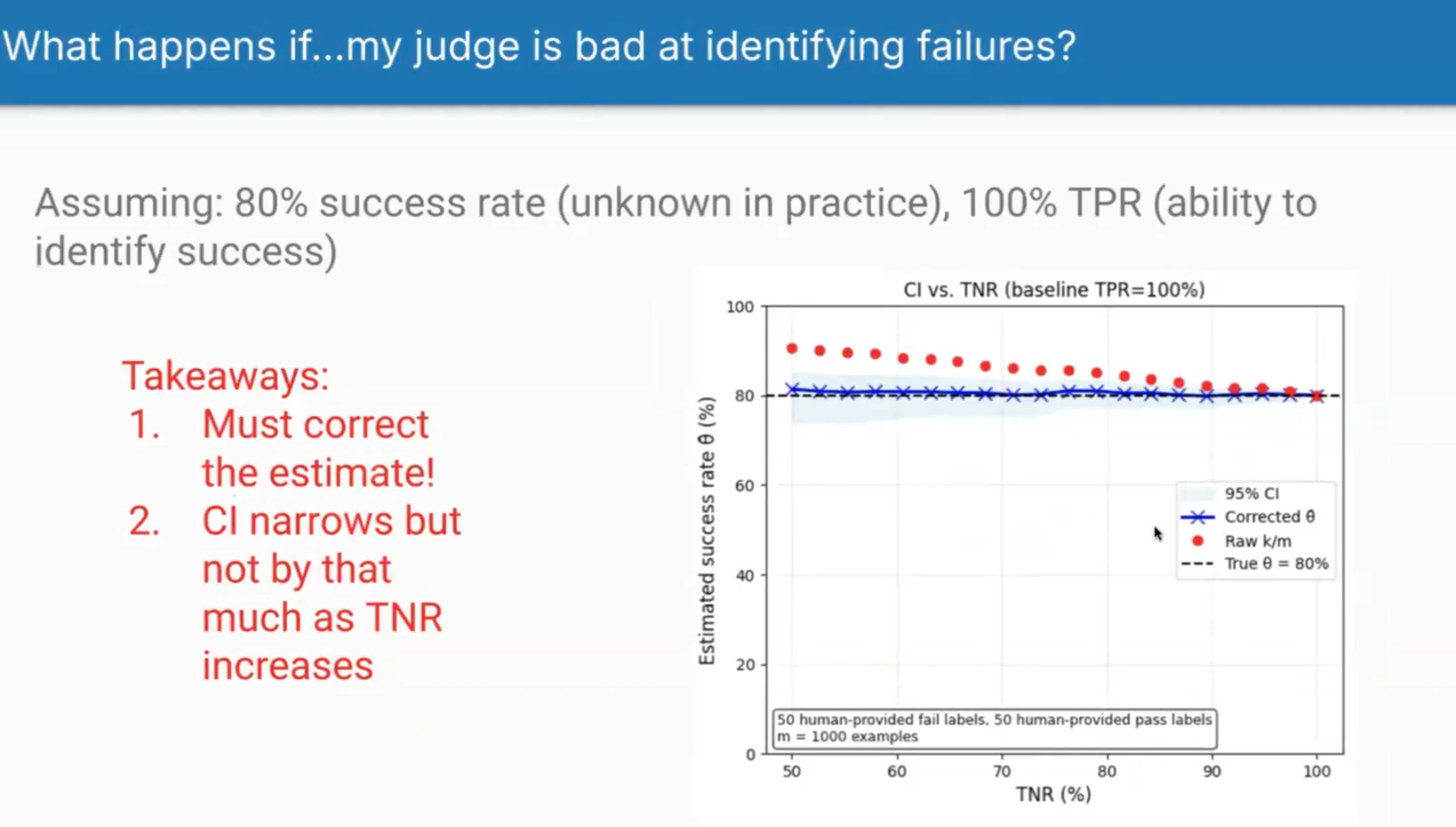
When judges are overly lenient (poor TNR), they systematically overestimate success rates. Shreya warned this is a common failure mode - judges biased to think everything is good, inflating success metrics that end up in dashboards and drive business decisions. If your judge has 60% TNR, you might see a 10% inflation in success rates, which could lead to false confidence in your system’s performance.

They’ve open-sourced a Python library called judgy that implements the bias correction mathematics, making it straightforward to apply these techniques.

Common Pitfalls

The lesson concluded with pitfalls to avoid:

1. Misaligned metrics - Evaluators that don’t actually measure what users care about
2. Over-confidence in scores - High automated test scores creating false security
3. Evaluator drift - Both model updates and changing quality definitions affect judges over time
4. Poor judge design - Missing few-shot examples or overly broad criteria
5. Skipping validation - The number one error: data leakage from using dev/test examples in prompts

thingsithinkithink

• The emphasis on narrow, single-purpose judges makes sense. It’s the same principle as unit testing - test one thing at a time so you know exactly what’s broken.

• The data hygiene requirements feel like overkill until you’ve been burned by meaningless metrics. I’ve heard of projects celebrating 95% accuracy that turned out to be testing on their training data. I can’t quite believe people do this, but I guess they do.

• Code-based evaluators deserve more credit. The reflex to throw an LLM at every evaluation problem wastes resources when simple checks would suffice.

• Tags:
• Llm
• Evaluation
• Machine-Learning
• Automated-Testing
• Course-Notes